Run PhyloVelo in C.elegans data

We next sought to benchmark PhyloVelo by applying to the phylogeny-resolved scRNA-seq data of C. elegans. The embryonic lineage tree of C. elegans is entirely known. Moreover, time-course single-cell RNA-seq data from C. elegans embryos has been mapped to its invariant lineage tree. We focused on the AB lineage which had the densest cell annotations from generation 5 (32-cell stage) to 12 (threefold stage of development), with mostly ectoderm and accounting for ~70% of the terminal cells in the embryo.

Data are available from Packer et al. at the Gene Expression Omnibus (GEO) under accession number GSE126954. Since multiple synchronous C. elegans embryos were pooled for the scRNA-seq experiment, many nodes on the embryonic lineage tree have been sampled multiple times. Only one cell was thus randomly chosen to represent the corresponding node, while these non-repetitive cells from one lineage tree constitute a “pseudo-embryo”. We focused on the AB lineage (the largest lineage amongst the first five founder cells contributing over 70% somatic tissues of C. elegans) and filtered out the genes with total count < 10 (remaining 6533 genes and 298 cells in a single psedo-emberyo). For the dimensionality reduction embedding of the scRNA-seq data, we used the UMAP embedding coordinates from original study13, which is available from https://github.com/qinzhu/Celegans_code/blob/master/globalumap2d_Qin.rds.

import pandas as pd
import matplotlib.pyplot as plt
import phylovelo as pv
import numpy as np
from scipy.stats import spearmanr
from mpl_toolkits.axes_grid1.inset_locator import inset_axes

import data

import pyreadr
globalumap = pyreadr.read_r('./datasets/Celegans/globalumap2d_Qin.rds')
globalumap = globalumap[None]

cell_annotation = pd.read_csv('./datasets/Celegans/GSE126954_cell_annotation.csv', index_col=0)
count = pd.read_csv('./datasets/Celegans/pseudoembryo0_count.csv', index_col=0)
sample = count.index

Read data using scData and filter

sd = pv.scData(count=count, Xdr=globalumap.loc[sample], cell_generation=cell_annotation.loc[sample].lineage.apply(lambda x: len(x.split('/')[0])).to_numpy().flatten())
sd.drop_duplicate_genes(target='count')
sd.normalize_filter(is_normalize=False, is_log=False, min_count=10, target_sum=None)

Inference and project velocity into embedding

pv.velocity_inference(sd, sd.cell_generation, cutoff=0.95, target='count')
pv.velocity_embedding(sd, target='count', n_neigh=15)

/home/wangkun/miniconda3/lib/python3.9/site-packages/phylovelo/inference.py:29: RuntimeWarning: divide by zero encountered in log
  pmf0 = -n_zeros * np.log((1 - psi) + psi * (n / (n + mu)) ** n)
/home/wangkun/miniconda3/lib/python3.9/site-packages/phylovelo/inference.py:29: RuntimeWarning: invalid value encountered in multiply
  pmf0 = -n_zeros * np.log((1 - psi) + psi * (n / (n + mu)) ** n)
/home/wangkun/miniconda3/lib/python3.9/site-packages/phylovelo/inference.py:29: RuntimeWarning: invalid value encountered in double_scalars
  pmf0 = -n_zeros * np.log((1 - psi) + psi * (n / (n + mu)) ** n)
/home/wangkun/miniconda3/lib/python3.9/site-packages/phylovelo/inference.py:333: RuntimeWarning: invalid value encountered in log
  y = np.log(y + 1)

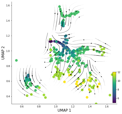
fig, ax = plt.subplots()
scatter = ax.scatter(sd.Xdr.iloc[:, 0], sd.Xdr.iloc[:, 1], c=sd.cell_generation, s=100)
ax = pv.velocity_plot(sd.Xdr.to_numpy(), sd.velocity_embeded, ax, 'stream',streamdensity=1.2, grid_density=25, radius=0.12, lw_coef=10000)
ax.figure.set_size_inches(8,8)
ax.set_xlabel('UMAP 1', fontsize=15)
ax.set_ylabel('UMAP 2', fontsize=15)
cbaxes = inset_axes(ax, width="3%", height="30%", loc='lower right')
plt.colorbar(scatter, cax=cbaxes, orientation='vertical')
ax.spines['right'].set_visible(False)
ax.spines['top'].set_visible(False)
ax.set_ylim([0.3, 1.65])

(0.3, 1.65)

Inference PhyloVelo pseudotime

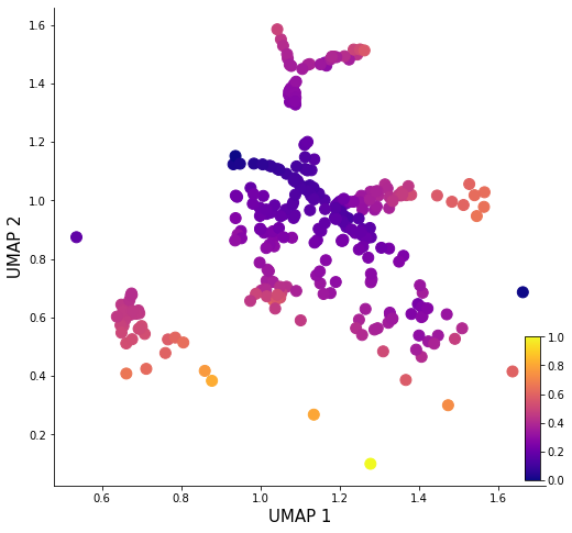
sd = pv.calc_phylo_pseudotime(sd, n_neighbors=280)

fig, ax = plt.subplots()
ax.figure.set_size_inches(8,8)
scatter = ax.scatter(sd.Xdr.iloc[:,0], sd.Xdr.iloc[:,1], s=100, c=sd.phylo_pseudotime,cmap='plasma')
ax.set_xlabel('UMAP 1', fontsize=15)
ax.set_ylabel('UMAP 2', fontsize=15)
ax.spines['right'].set_visible(False)
ax.spines['top'].set_visible(False)
cbaxes = inset_axes(ax, width="3%", height="30%", loc='lower right')
plt.colorbar(scatter, cax=cbaxes, orientation='vertical')

<matplotlib.colorbar.Colorbar at 0x7f94b5eb0f70>

x = cell_annotation.loc[sample]['embryo.time'].to_numpy()
y = sd.phylo_pseudotime

a, b = np.polyfit(x, y, deg=1)
y_est = a * np.linspace(50,650,60) + b

fig, ax = plt.subplots(figsize=(7, 6))
ax.scatter(x, y, alpha=0.4, s=70)
ax.plot(np.linspace(50,650,60), y_est, '-', c='k')
ax.set_xlabel('Embryo time', fontsize=17)
ax.set_ylabel('PhyloVelo pseudotime', fontsize=17)
# ax.text(50, 0.9, 'spearmanr={:.2g}\np_val={:.2g}'.format(*spearmanr(x, y)), fontsize=15)
rho, pval = spearmanr(x, y)
ax.text(50, 0.98, r"Spearman's $\rho$={:.2g}".format(rho), fontsize=15)
ax.text(50, 0.91, r'$p={}\times 10^{}$'.format(*r'{:.2g}'.format(pval).split('e')).replace('^', '^{').replace('$', '}$')[1:], fontsize=15)
ax.spines['right'].set_visible(False)
ax.spines['top'].set_visible(False)